ML Engagement
Report —
Intellipieux

This report summarizes the audit done of the 2025-05-13 Intellipieux report (Previous Report) and subsequent improvements brought in during the span of a collaboration led by Prof. Dr. Jean-Baptiste Payeur, featuring Probabl and Logilab.

The Previous Report served as a basis of understanding for the problem to solve and the available data. Along with it, a dump of pre-processed data was delivered, starting with a file training_data_2025-03-27.csv and later a file training_data_2025-12-01.csv with updated data and improved preprocessing.

We point out that said pre-processing includes some transformations that might be non-neutral with respect to the downstream tasks. For instance, although the raw timeseries were recorded as functions of time, the given dataset pre-processes it into functions of depth. This transformation is not injective and involves assumptions and choices, especially when needing to select a unique value for each given depth, while back-and-forth drilling sometimes registered several different values. This pre-processing thus alters some of the information. At first glance, it looks safe, but we wondered if the question of its necessity and impact could be investigated more carefully. In-depth exploration of this was not in the scope of the project and we chose to build directly on what was given regardless.

The Previous Report provides a good introduction to the business context and an overview of all measured parameters during drilling, and provides plots of value ranges. We proceeded to additional data discovery and inspection using skrub.TableReport. We also implemented a module intellipieux.models.data that includes a data validation layer validate_drilling_data that runs a sequence of healthchecks on the provided dataframes of raw data. It checks for types, duplicates (after building a strong index to ensure unicity of samples), and consistency between metadata and drilling data. In particular, it detected issues in training_data_2025-12-01.csv that were immediately reported and fixed. The validation layer is also used to validate inputs for the live service, showcased in the dash demo, and will exit early if it detects corrupted data.

We decided to rename some of the variables within the data validation layer, in favor of more explicit and readable names, so as to enhance clarity of the code assets that were produced during the study. Here is the mapping table:

where Initial is the column of variable names introduced in the Previous Report and used in the provided CSV, and New are the names that we used instead.

From then on, the mission consisted in taking over existing work aiming at modeling the variations of the bearing capacity as a function of the real-time drilling parameters measured by a drilling machine, so that the depth of the piles of concrete can be minimized for a given compliant bearing capacity, and save on concrete by beating estimates made by expert geologists. The downstream metric of success is the financial gain made from concrete savings.

The Previous Report previously broke down the capacity prediction into the prediction of two components: shaft resistance (with notation Qs or bearing_capacity_(lateral)) and tip resistance (with notation Qp or bearing_capacity_(tip)), with shaft resistance being the most important component, and tip resistance being expected to be harder to model. We prioritized towards modeling shaft resistance. Study of tip resistance could not be started in the timespan of the project.

For shaft resistance, we audited existing work reported in the Previous Report and browsed the corresponding implementation, then achieved a similar roadmap while addressing a number of issues and attempting to enhance the models. The roadmap included laying a strong methodological framework, an overhaul of the code assets, some feature engineering, hyperparameter search, estimation of prediction intervals, creation of reports, and providing a library to embed trained models into the real-time service.

Bearing capacity estimation is approached as a regression task. We aim at leveraging the dataset of drilling data and metadata, along with (somewhat inaccurate) estimates of bearing capacity given by different pre-existing estimation methods, so as to be able to predict bearing capacities for new unseen drilling data.

The true bearing capacity values come from several different sources, that have possibly significantly different measurement errors and artifacts. At the moment, the dataset includes samples obtained with two methods: CPT and PDA. The Previous Report provides a more detailed breakdown of their differences. Data extracted from other methods, such as SPT, appears to be unreliable, and was discarded upon more accurate inspection.

Both methods delivered true bearing capacity estimates of concrete piles built in several construction sites. On top of that, both methods also delivered estimates of bearing capacities at intermediate depth, as if the piles had really been drilled at inferior depths. CPT is expected to be equally reliable for estimations at true and intermediate depth. We do not have such an a-priori expectation for PDA estimates.

The true target of interest is the bearing capacity as given by the PDA method for the existing concrete piles at their true depth. However, since the PDA data at true depth is scarce, we hope for better training by including all data in the training set, including CPT estimates, and all estimates at intermediate depths. In order to learn to predict the target, the models can use information about the estimation method (CPT and PDA) and about the depth of the measurement (intermediate or true depth, with respect to the real concrete piles). During real-world usage, the measurement method we want to predict will always be PDA, and the prediction will always be at a depth that is assumed to be the depth of the real concrete pile that would be poured.

The Previous Report mostly reports RMSE, while the corresponding implementation both showcases RMSE and MAPE; similarly we did also report RMSE and MAPE. For models that leverage all data (PDA and CPT, including intermediate depths) we report those metrics on the whole dataset, but also on each disjoint subset of samples belonging to PDA or CPT, at true or intermediate depths. Metrics over samples given by PDA at true depths are the most accurate depictions of the task being addressed, however are less likely to generalize because of the small number of such samples. Global metrics and other subsets give additional insights, with different amounts of variance and biases.

One issue with RMSE and MAPE is that they only give insights for average performance. However, estimation of bearing capacity is much more sensitive to overestimation of the true target, and much less to underestimation. Overestimation of the bearing capacity would result in too short drills and too weak piles, at best incurring additional costs and delays for re-drilling, at worst threatening the integrity of buildings. In fact, the cost of overestimating bearing capacities can be considered infinite.

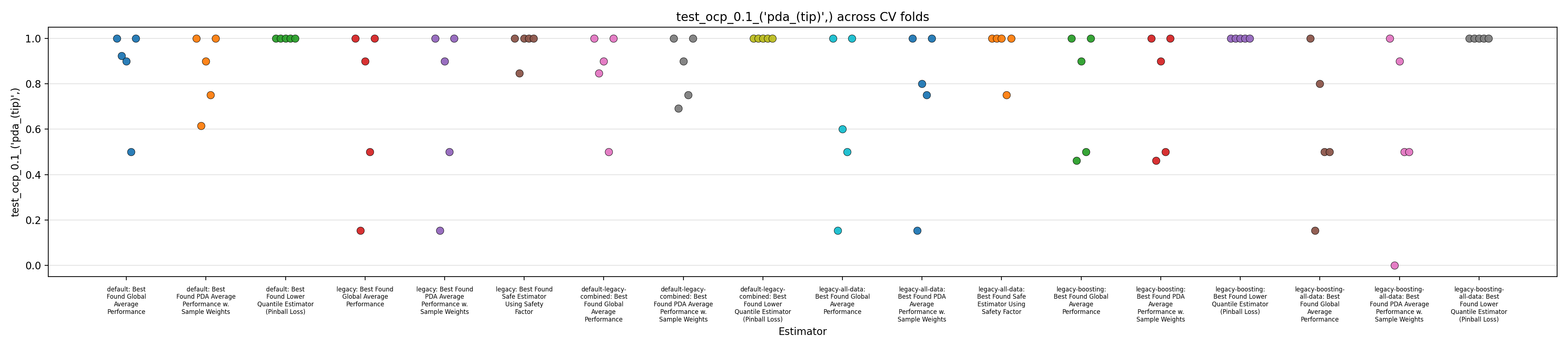
Thus, it is crucial to also report metrics that evaluate the risk of overestimation. We introduce OCP@tol, for Overestimation Complement Percentage @ tol, which is equal to the fraction of the data for which a model does not overestimate the target by more than tol x 100 percent. A value of 1 means no overestimation (in the limit of the tolerance tol), 0 means only overestimation. We report OCP@tol for tol=0.05, tol=0.1 and tol=0.2

We want to select models that have the best RMSE or MAPE, provided some set minimum value for OCP@tol for some given value tol, below which models will be discarded.

Finally, the Previous Report also evaluates the amount of saved concrete, and subsequent financial gains, by comparing the predictions with those of expert geologists. In the timespan of our contribution, we did not have access to the specifications from the geologists and unfortunately could not continue producing this metric.

Machine Learning models are prone to overfitting, meaning that after being trained, a model performs better on the data it has been directly trained on. Performance on the training dataset does not usually translate fully to performance on unseen data. That is why we hold some data out of the training set, so that it remains unseen at training time, and report metrics computed only on this separate data. Those two separate sets of data are typically called "training split" and "validation split".

The Previous Report did indeed put in place such an evaluation framework. But there are a few more pitfalls when setting up proper evaluation methodology, and we identified at least two that it fell into, that could have undermined the conclusions.

The first one is a form of data leakage: the validation dataset was made of data extracted from a single given construction site, however it says that 25% of the data of said construction site was included in the training dataset instead. From reading information about local geological profiles provided in the Previous Report, we suspect that knowledge of a single pile in a construction site provides predictive information for all other piles in the vicinity, and maybe even all the piles for the site to some extent. But in real-world usage, models will be used on new construction sites where all piles were completely unknown at training time. Thus, validation metrics should be reported on data from construction sites whose piles never appear in the training set at all, or face the risk of displaying an overly optimistic picture. Maybe this assumption could be limited to concrete piles close to each other (that we could control using provided longitude and latitude) rather than coercing to all piles of a same construction site, however we chose the most cautious approach for the time being.

The second one is related to the scarcity and inaccuracy of data in this project, that let us assume that the signal-to-noise ratio is low. We fear that reports of performance on a single validation split might not provide insights that will generalize well enough to real-world usage. We could be observing results explained by a statistical fluke, rather than by the power of the model. A common mitigation in this case is to repeat train/report experiments, with different choices of train/validation data splits, a method also called cross-validation. This approach, run with 5 different splits, indeed showcased important variations in reported metrics, depending on the split, ranging from one to two times the rate of reported errors. From then on, all reported metrics and figures are displayed for each of the 5 splitting strategies, so as to highlight the variance, and especially the distance between best case and worst case scenarios.

One can see that the implementation has to account for many intricacies: complex merges in timeseries of unequal lengths, cross-validation with non-overlapping groups, custom metrics on subsets of data, prediction intervals (overestimation control), real-time service on new data, and ambition to showcase a benchmark that compares approaches described in the Previous Report and novel approaches, all while ensuring reproducibility, and solid foundations for future iterations. Our final deliverable counts about 2000 lines of Python code.

The code that sustained conclusions of the Previous Report was handled in a collection of Jupyter notebooks, and later converted to a Python executable using nbconvert. We warned that such a development environment will not adapt well to the complexity of the project, and we transformed it into a more standard tree of modules within a Python app. Here is the resulting module tree:

.
├── baseline
│ ├── features.py
│ ├── __init__.py
│ └── models.py
├── data
│ └── __init__.py
├── features
│ └── __init__.py
├── __init__.py
├── __main__.py
├── metrics
│ └── __init__.py
├── models
│ ├── __init__.py
│ └── wrappers.py
├── reporting
│ └── __init__.py
├── service
│ └── __init__.py
├── stats
│ └── __init__.py
├── train
│ └── __init__.py
└── utils.py

with the single endpoint command that orchestrates the training step python -m intellipieux.models with the following interface (displayed by running python -m intellipieux.models --help):

usage: __main__.py [-h] [--output-path OUTPUT_PATH] [--output-prefix OUTPUT_PREFIX]
[--random-state RANDOM_STATE] [--n-splits N_SPLITS]
[--capacity-measurements-min-depth CAPACITY_MEASUREMENTS_MIN_DEPTH]
[--cachedir CACHEDIR]
[--model-strategy {default,default-legacy-combined,legacy,
legacy-all-data,legacy-boosting,legacy-boosting-all-data} [...]]
data_path

and the module intellipieux.models.service implements the interface for live predictions.

The code architecture was also brought to better standards with idiomatic usage of all of the scikit-learn toolbox. In particular, we implement an ad-hoc data querying layer with a data model adapted to drilling timeseries, and make use of metadata-routing to route the data layer interface, as well as metadata, to the relevant objects. An effort was also sustained to improve inline readability with explicit variable names and comprehensive docstrings.

The training command, when used with a small subset of data, can enable quick local validation that things work as expected. We were however lenient in unit testing, as well as enforcing coding style constraints, and those areas could be improved in the future.

Much like the models described in the Previous Report, the features extracted from the data leverage some of the metadata (type of pile, diameter, height of platform, real depth of the pile, type of measurement, depth of measurement, ...), and the drilling timeseries. We summed across all depths a few select quantities that combine different timeseries: force_thrust / advance_speed and rotational_torque_bar / rotational_speed. The latter had already been found by the Previous Report to be relevant to the model. The first is similar but for the vertical component, rather than the rotational component. Only a few combinations of features could in fact be used, judging by reports of missing values, with many variables being completely unrecorded, or only available for half the construction sites in the data.

On top of that, the Previous Report explored more elaborate feature engineering ("trend" features), that we ported and had to optimize, because the quadratic complexity found in the provided implementation only enabled training on very tiny subsets of data, and did not scale to training on the whole PDA+CPT dataset. We could not however conclude any significant performance improvement brought by this strategy, compared to our "sum-over-z-axis" initial approach.

We also added some standard normalization steps on top of the extracted features, and optional feature selection using a Ridge linear model.

Clearly, there is room for a much more ambitious exploration of strategies to extract signal from those timeseries, and, we hope, for significant performance improvements. Much of our contribution consisted in validating and sanitizing the experimental framework, and we could not also address such in-depth exploration of features in the given timespan. We could, however, review the relevant state-of-the-art: low-hanging fruits could consist in leveraging on-the-shelf feature extraction transformers, from libraries such as sktime, aeon and tslearn, in particular standard catalogues of features such as catch22 and tsfresh, or convolution-based or other local-based approaches such as MiniRocket (and in particular the multivariate ones) or shapelet-based approaches. We only started a very preliminary exploration of the Catch22 features that unfortunately did not display meaningful changes, but we also did not study enough to commit to conclusions.

Besides, Prof. Dr. Jean-Baptiste Payeur gave hints towards a quantity that has been described in geological state-of-the-art journals, called Normalized Penetration Ratio (or NPR), roughly equivalent to rotational_speed * ((diameter / force_thrust)^alpha) for some value of alpha (suggested to be close to 0.1), as providing significant information regarding ground resistance, that we should also try to leverage in future iterations.

One could also consider building features out of limited local drilling data at the depth where predictions are made, rather than trying to include the whole drilling timeseries from base to prediction depth.

Our feature extractors might also benefit from improvements on basic good practices, such as systematic detrending and smoothing.

We ran a histogram-based boosting regressor on top of the extracted features, and a grid-search over hyperparameters, especially parameters related to regularization. This strategy is a common, solid baseline that will commonly yield decent results out of the box. We also compared with the LinearRegressor that was seen in use in the Previous Report and could show that HGBT performs better overall.

Lately, a new hot trend has emerged for classification and regression for small datasets: transformer-based tabular foundational models, see for instance tabiclv2. Those models do not require tuning, and are reportedly easily and consistently netting significant (yet still within incremental ranges) performance improvements over baseline boosting strategies. Their downside is that they require more powerful hardware including GPUs, and could be more expensive or slower to operate at inference time. Still, it should be added to the roadmap of improvements to investigate.

We also explored leveraging sample weight strategies, so that the loss that is optimized penalizes errors more if they are relative to targets obtained from PDA measurements or from PDA measurements at true pile depth. We could not conclude any meaningful improvement. It is a cheap addition that could however still prove valuable to get a few extra performance points in the future, were we to manage to improve the model in other aspects.

We also reviewed extensively state-of-the-art strategies for interval prediction, and especially to optimize for best average performance (given by RMSE, MAPE metrics) while controlling for the risk of overestimation.

The Previous Report introduced a post-processing step over the values given by the average regressors, that consists in multiplying by a constant safety factor. We point out that Figure 21 "Definition of model factor. Image generated with the help of ChatGPT" is misleading in this regard, since it displays a translation of the decision thresholds as if the safety factor was additive, but it is in fact multiplicative, meaning that the absolute difference after safety correction depends on the magnitude of the predicted bearing capacity. We ported the safety factor strategy, and improved the selection of said factor by running a parameter grid search with cross-validation, using RMSE and MAPE metrics conditionally to some threshold value of the OCP@tol indicator.

State-of-the-art review for risk control in regression gives, in fact, a palette of other strategies that could be comprehensively reviewed to get the safest predictions, while keeping the RMSE and MAPE at an acceptable level.

One of those consists in optimizing the pinball loss rather than the squared error, for some given target quantile, which is supported by our baseline HistGradientBoostingRegressor model. The advantage of this approach is that it yields prediction intervals that account for the values of input features, and thus are sample dependent. It acknowledges that there are areas of the feature-space where predictions should be more cautious, and areas where it can be more confident (this is called assumption of heteroscedasticity, as opposed to homoscedasticity). We did run this strategy for our best average model, but only to report a disastrous drop of RMSE and MAPE. One explanation could be that strategies that make the heteroscedasticity assumption require a lot more data to train properly than we currently have. Another explanation could be an error in our implementation: instead of recycling hyperparameters from our best average model found with squared error, we should have run hyperparameter search from scratch specific to the optimization of the pinball loss. The latter might very well be the explanation, as we thought to recall having showcased before acceptable results that leveraged the pinball loss. Unfortunately, we lacked time to finish this investigation. Last but not least, under the assumption of heteroscedasticity, the distance between the average prediction and the safe prediction can also be leveraged to quantify the uncertainty for a given prediction.

Under the assumption of homoscedasticity, it could be worth exploring an additive correction to the prediction, instead of multiplicative.

More generally, a reference, on-the-shelf library for risk control is MAPIE. However it relies on split-based cross-validation strategies but is not yet able to account for non-overlapping groups out-of-the-box, hence leveraging this library will require non-trivial integration work.

We close this report by displaying figures showing performance across the 5 splits in a cross-validation setup.

The performance of 6 models are reported:

• "default": our own baseline model that was developed independently of the Previous Report.
• "legacy": our reproduction of the model described in the Previous Report, ported using mostly the implementation found in the Jupyter notebook.
• "default-legacy-combined": like 'default', but the trend feature from the 'legacy' model is added to the list of features.
• "legacy-all-data": like 'legacy', but trained on the whole dataset, rather than just 'PDA' data.
• "legacy-boosting": like 'legacy', but the linear regressor is replaced by a histogram gradient boosting regressor.
• "legacy-boosting-all-data": like 'legacy-boosting', but trained on the whole dataset, rather than just 'PDA' data.

Each of those 6 models are evaluated in three different setups:

• normal training, with uniform sample weights
• normal training but selecting the best among several strategies of sample weights
• after correction to prevent overestimation (using pinball-loss optimization for boosting, or the "safety factor" for linear models)

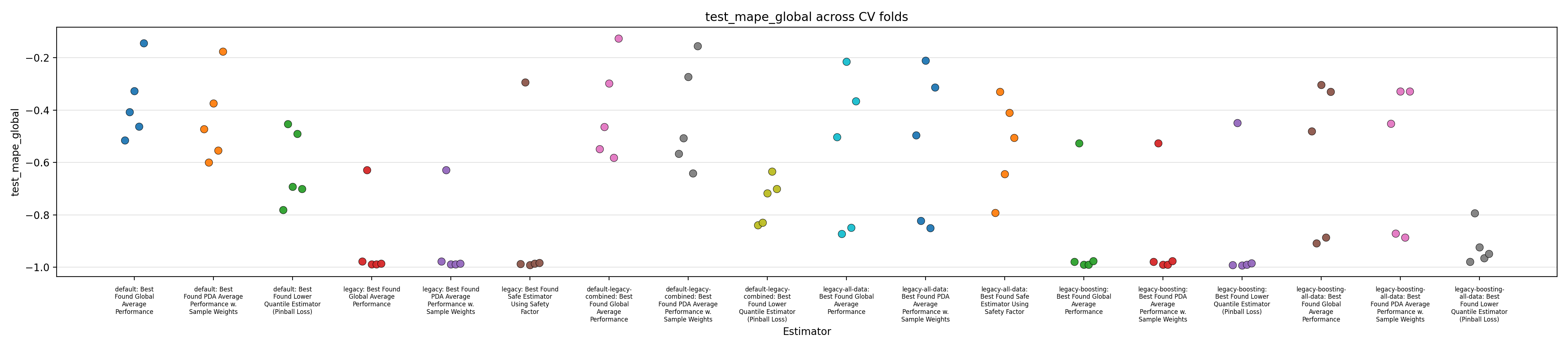
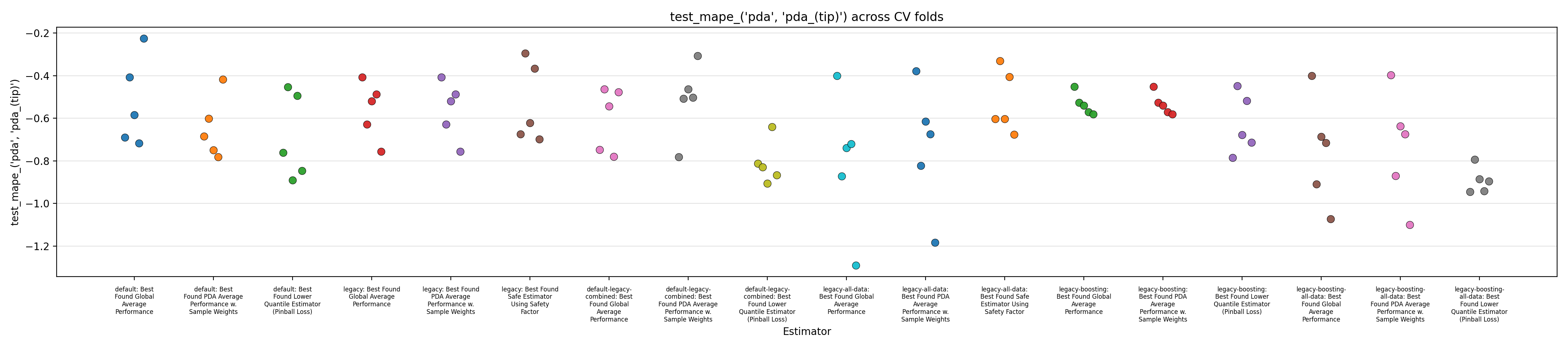
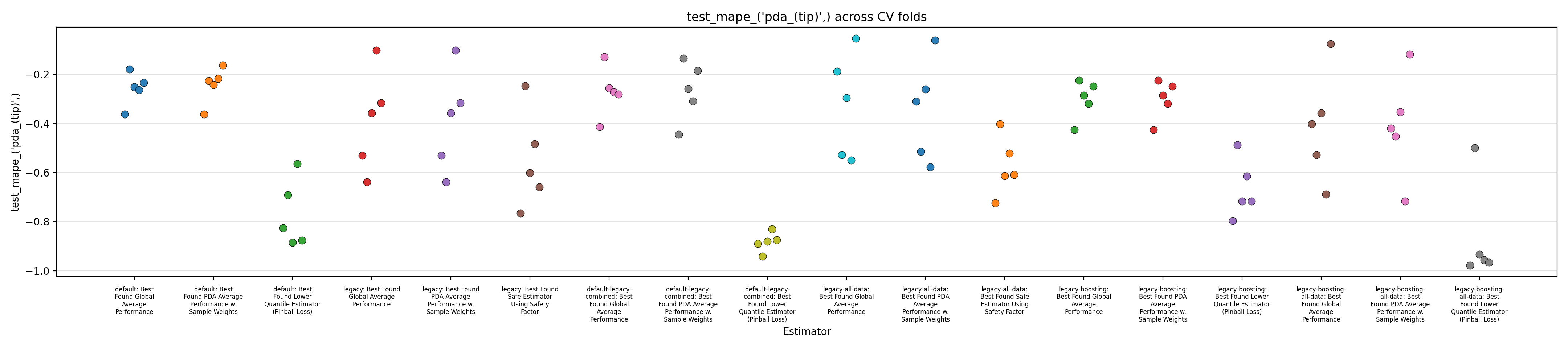
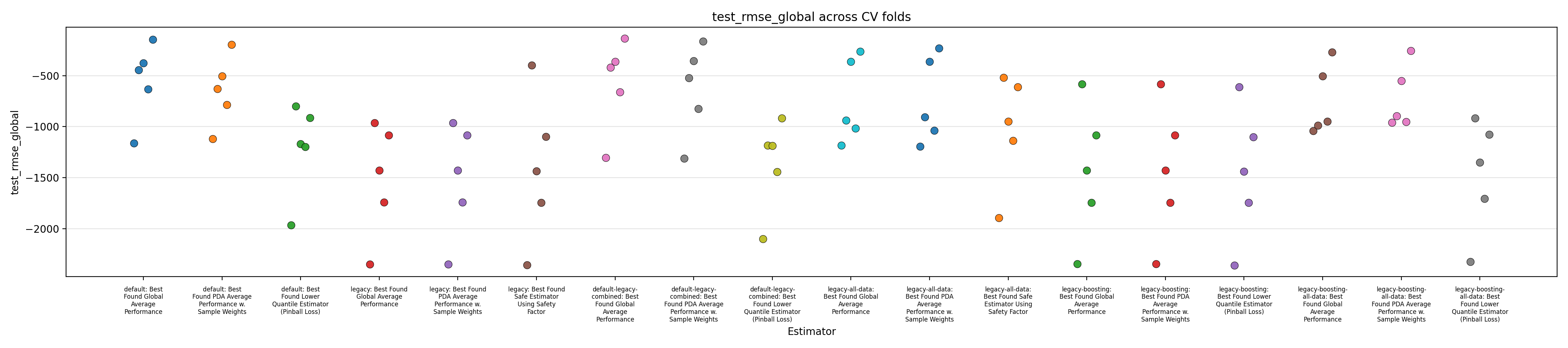
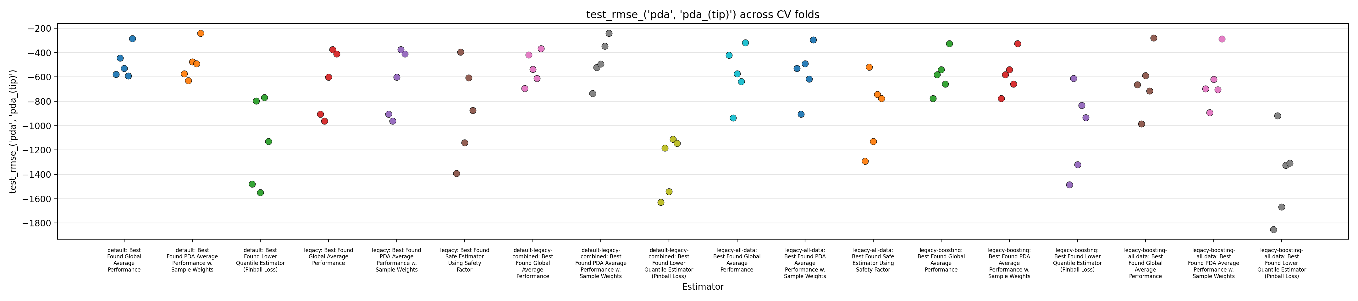
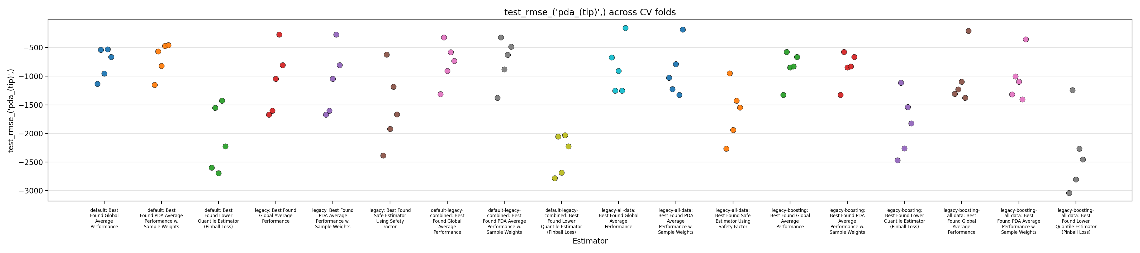
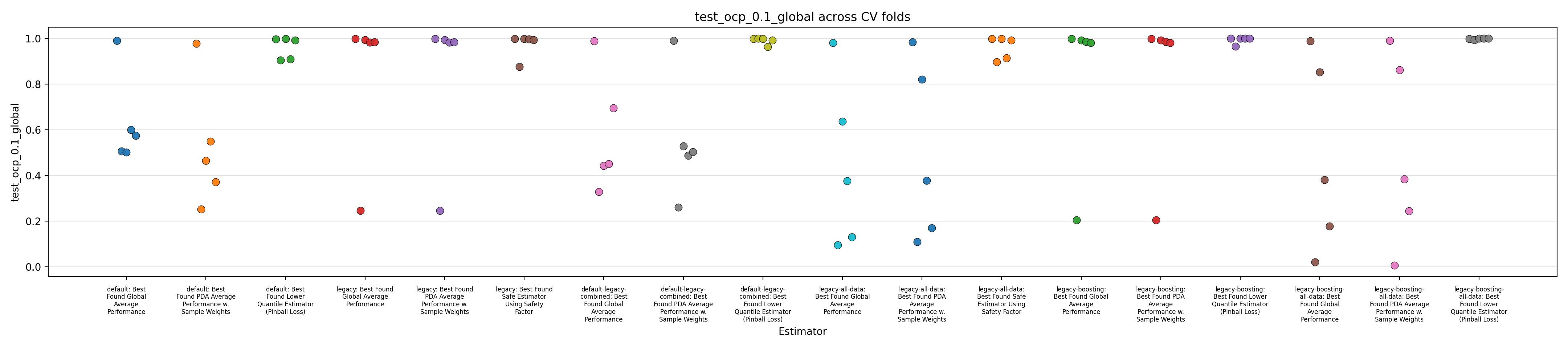
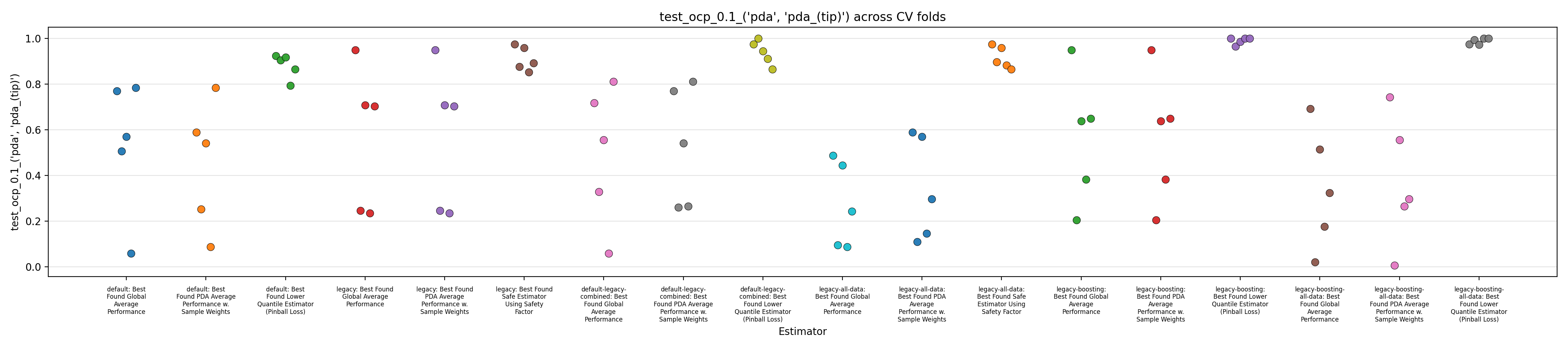
Figures 1 to 3 display the MAPE on validation splits across CV folds, on different subsets of data: respectively MAPE averaged over all data, or only PDA-related data (including estimation at intermediate depth), or only PDA-related data at true depth. Figures 4 to 6 display the RMSE rather than MAPE. Figures 7 to 9 display OCP with a tolerance of 10% overestimation.

It is obvious that for all models, metrics observed across the different splits are very scattered, with for instance MAPE range having about 0.5 width, for about every model, with our default model appearing to average slightly better performance across the board, along with the legacy strategy (using the trend features and limiting training to PDA) coupled with boosting. It confirms the weaknesses of evaluation methodology suspected in the Previous Report.

The safe corrections for the boosting models, however, display an important loss of performance, indicating that the pinball loss strategy was not effective at controlling overestimation without degrading average performance. However, linear models corrected with the safety factor do keep displaying some cases of overestimation.

Overall, those figures indicate high instability and go against the idea that it could be leveraged into a viable business use case. This could be confirmed by comparing the safe models with estimations from the expert geologists, and reporting the amount of occurrences where it is beaten, which are expected to be low. However, some signal still seems to have been captured by the models and does not dismiss any possibility of improvement. One could foresee that increasing the quantity of available data, and continuing effort at more elaborate feature engineering, could stabilize performance and make the product viable.

Figure 1 — Global MAPE

Figure 2 — MAPE on PDA data

Figure 3 — MAPE on PDA data at true depth

Figure 4 — Global RMSE

Figure 5 — RMSE on PDA data

Figure 6 — RMSE on PDA data at true depth

Figure 7 — Global [email protected]

Figure 8 — [email protected] on PDA data

Figure 9 — [email protected] on PDA data at true depth